Project 3: Landslide Hazard Map – inverse modeling – EEG 260

This project has you create another landslide hazard map using slope and aspect as before, but now including the predictor variables of landform shape (curvature) and geology in addition to slope and aspect. Find one or two new partners for it. The biggest difference with this analysis will be using the location of actual landslides that occurred in 1995 to train the GIS to recognize areas of potential future hazard in an inverse model approach.

You will be completing this lab as a large layout that will be posted and discussed during a future class as a way to learn about how to best communicate GIS analyses. Your hypothetical audience is the Town Council for the Cities of Buena Vista and Glasgow, and the Rockbridge Board of Supervisors. They are looking into landslide hazard zoning regulations, or possible protective measures, and they need your expert services. Your goal is to come up with an answer that can be explained to non-technical, but intelligent people in a poster-sized presentation; part of our emphasis for this project is learning to display both GIS processes, plus data and results, clearly and accurately.

Do this lab with one or two other students.
Here is an outline of the steps.

Data and preparation
1. Copy the folder containing necessary new data R:\courses\GEOL260\sharedwork\Projects\Project3
2. Create a new project in that folder.
3. In the catalog, locate, import or copy the necessary data from previous projects and exercises (~~take a minute to update any feature or grid metadata to show its origin~~), including
  1. a 1 arc second (about 30 m) DEM (projected but not clipped to previous project study area polygon, because that is not be enough territory for the landslide frequency). NOTE: the DEM should be projected to UTM 17 NAD 83 and the projection should be done with bilinear or cubic convolution resampling, not nearest neighbor (check the metadata if you’re not sure). If you’re unsure of the important “first step,” ask for help. Or use mine from the Project 3_22.gdb
  2. maybe… the BV/Glasgow topographic map image (from the geology tile georeferencing (or you can use the “background” USA Topos layer.
  3. Geology (Dave’s “repaired” geology data or one of your own doing). You will want to convert this to a grid that matches the cells of the UTM NAD 83 DEM (cell size, raster snapping). This layer is located in the Project3 geodatabase in the R drive and a backup shapefile in case the gremlins are active today. Note that the dataset still has errors but they shouldn’t pass through to the resulting grid. Let me know if that’s not true.
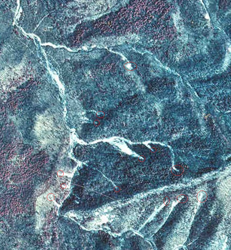
Digitize the 1995 landslide “headscarps”
In 1995, the Glasgow Blue Ridge area received about 18 inches of rain in 2 days! Landslides occurred in the steep terrain around Glasgow and going north toward BV. Your job is to find and map as many of them as you can to use as a training set for the inverse model.
1. Open the “orthophoto” for the SE part of the Glasgow Quadrangle (USGS Orthoimagery) that I placed in the project3 folder (it is from R:\orthophotos). Note: the BV orthophotos do not show landslides.
  The overlap between the geology, DEM, and orthophoto is considered the “training area” for this inverse model. Whatever occurs in this region is the input for the likelihood prediction for the rest of the geology/dem data.
2. From this quarter-quadrangle, digitize the landslide headscarps as points. They are circled in red below and you can also see the path taken by the ensuing debris flow (blue), some of which took out bridges and one nearly made all the way to the Maury River.
  
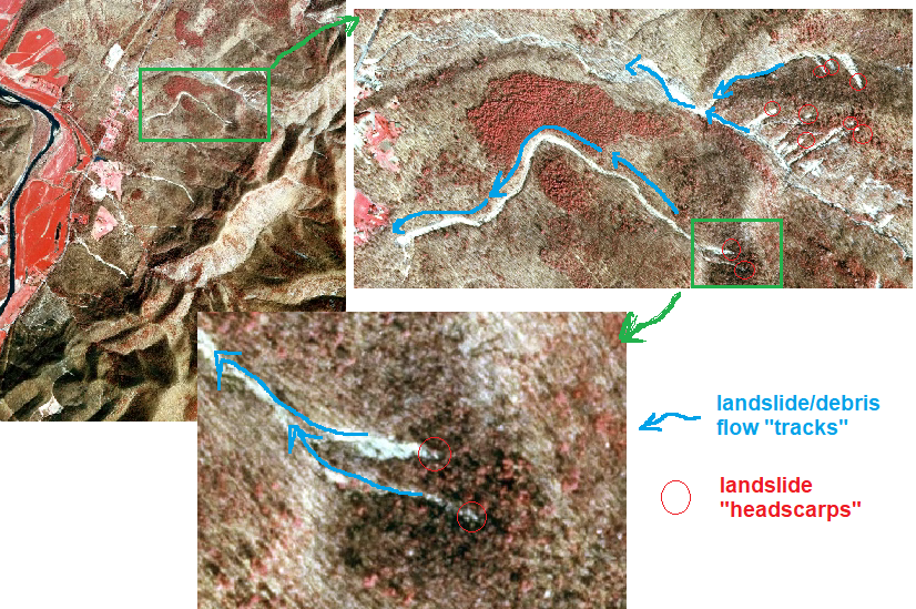
  It is impossible to tell how large the sliding area is now, because evidence of the lower limit was removed by flow downhill after the slide starts. So a point or very small polygon area of the headscarp area is the best model for landslide initiation. When you’re done, evaluate the accuracy (mostly thematic) and precision (mostly, how well located, in m) of this endeavor (both categorical and spatial) and put that in the metadata. Precision should be a number, in meters, not “really good.” 🙂 Categorical? How certain are you that all your points are landslides? Not everything that is “white” here is a landslide. See the bottom of the image where the cliffs and “taluses” are NOT circled.
Create the inverse hazard model
1. Create a new geoprocessing model for the landslide hazard, pull in the DEM, Geology and new landslide headscarps (projection? cell size? snapping? extent?)
2. Assemble/create landslide and landform attribute layers (slope, aspect, curvature) for analysis and display.
  1. Do some of the landslides need to be larger than one cell? (30×30 m) You can buffer some of them that are larger, or all of them to account for uncertainty. No right answer here.
  2. Make the landslide point data and/or buffer data into raster file.
  3. Landform Predictors:
    1. Slope as before, indexed somehow?
    2. Aspect, for sure, and indexed?
    3. Geomorphologists like Dave will tell you that landslides form in “hollows” above first order streams where soil and water create the conditions for slides. Is that true here? Curvature is the metric to investigate. Take a look at the different curvature possibilities and make a choice. Do look at the histogram of curvature before you decide how to index it (strongly nonlinear distribution).
  4. Note that rainfall would be a great layer to have, but I don’t have any data from that storm.
  5. Geology. (question: does using slope and geology violate our “independence” rule for Bayes factors? Go ahead and use both but worth thinking about the statistical rules one violates or not…..)
3. Perform inverse modeling (an “overlay”) on these possible contributing layers (slope, aspect, elevation, curvature, geology, add anything else you want for extra credit). We are counting the frequency of landslides within the above “training area.”
  1. Analyze the distribution of the slides (either as a map or a table) within the categories of each of the predictor variables.
  2. Geology is already a categorical layer. What will you do with the others? The process shouldn’t unfairly accentuate or diminish one predictive layer vs another.
  3. Do you want output maps? Tables? Think it through. What is the best way to communicate this.
Predict future landslide hazard using the inverse data
1. Use the output of the overlay analysis to create weighted indices of hazard for future landslides.
  1. Use the count/sum of landslides per category of each predictor to assess the hazard. The frequency itself is a measure hazard in a particular zone (or as shown below where the count becomes a 0-10 “index” using simple division), but the best is to use Bayes probability modeling to get the posterior factor for each predictor category (doing the Bayes probability modeling would be extra credit +10 if well done).
  2. If you use indices, do you need to weight? Or is the process of finding landslides and their counting enough. Think about it.
2. If you use the Bayes process (+10 pts extra credit), you will be producing “posterior factors” that you can sum or multiply for different the different predictors. Think about what the “T” area should be as illustrated above. It is not the full area of the geology map or study area, it is just that area that is covered by the image with the landslides on it.
Create a poster layout that is 24″ x 36″ with map frames, text, and other elements showing the important processes of the analysis.
1. finish your analysis before you start playing with a final layout.
2. use overview and/or zoomed in maps, annotations, words, colors, and/or arrows in a simple yet complete poster that shows the folks of BV your hazard analysis.
3. limit the use of GIS jargon (the audience is intelligent but not ArcGIS literate)
4. Once the model works, make sure it has sufficient labels. You are welcome to export it as a graphic and use it in the layout, but remember your audience. If you do use it, you are free to modify the model description using any other program to add explanation or documentation before sticking it on the poster layout (you can add images, etc to a layout).
5. Display any data/analyses you deem necessary over a basemap, shaded relief, or hillshade.
6. You likely need a bit of text on how your process works to isolate the areas of landslide risk. This should explain the hazard above dwellings or structures in areas of interest to your client(s). Words, charts or maps.
7. Export the layout to a pdf in your project folder.
Metadata: Metadata should be on the input data, but your model is most of the metadata for the process. Make metadata for the final hazard grid(s) or feature class(es) that refers generally to the outline of the process and the name and location of the model used. Let’s not take the extra time for metadata except for the landslide headscarp feature class.

Make a new portfolio that has the following

- the authors
- a brief letter to the city and county officials who requested your analysis
- ~~a list of data that should have metadata in the catalog~~
- The PDF of the layout
- a snip of your landslide model (make sure it is legible)
- snip of the landslide metadata as seen from the TOC properties panel

In Canvas, report
– the group member names,
– the link to ONE portfolio I should consider,
– the filename and path of the exported PDF layout, and
– the location and name of ONE ArcGIS Pro project I should consider (in P or Q) if needed.

Evaluation Criteria (75 pts total):

	pts	Excellent	Good	Fair	Poor
Digitizing	15	13-15 –all or nearly all landslides well-placed	10-12 –some location and/or content error, more than a few missing points	7-9 – only some landslide points in ok location	<7 – landslides missing or mostly improperly identified
Landslide model	30	25-30 – well-documented (with labels) and well-composed model with appropriate analysis and output. Yields landslide potential based on a clever indexing of counts from 1995 storm.	20-25 – Effective inverse model with simple output that includes reasonable indices for landslide hazard. Some documentation missing on model.	15-19 – Simple inverse model with correct results and some documentation.	<15 –model incomplete or does not produce correct results
Poster Content	15	10-15 – the poster fully presents the GIS data and process without unnecessary detail.	8-9 – most of the important steps are present and clear	6-7 –poorly organized or missing/ muddling/ too much info for presentation of data or process	<6 – poster elements do not effectively portray the GIS data and process
Poster commun-ication	10	10 –maps and text are clear and well composed. All maps have necessary marginalia. Text is necessary and brief.	8-9 –good map and text components, but contains unclear or incomplete information or text	6-7 – missing some map information (legends, titles, scales, etc) and/or text is missing, insufficient, or excessive.	<6 – map and text components are incomplete and fail to provide necessary clarity to process.
Metadata and portfolio	5	5 – metadata made for original and digitized layers and final hazard map; portfolio has requested info	4 – something is missing	3 – one than one something is missing	<2 – no metadata or doc/path/filename submission failures